
Dislocation Dynamics
2.5-Dimensional Dislocation Dynamics
Discrete Dislocation Dynamics (DDD) is a simulation method developed to describe the collective motion of dislocations at the mesoscale and to address the intra-crystalline plastic behaviour in different materials and under different external conditions.
Dislocation motion is a complex phenomenon that involves breaking and distortion of atomic bonds close to the dislocation line, but also the deformation of an extended crystal region where the atoms are slightly displaced from their equilibrium positions. Linear elasticity theory allows one to describe the stress field induced by dislocations into the crystal lattice and, as a consequence, the force acting on each dislocation. The latter is the so-called Peach-Kohler force expressed by the following equation:
FPK = b . (σapp + σint) x l (1)
where b and l are the dislocation Burgers vector and line direction, σapp is the external applied load and σint is the stress field induced by the dislocation microstructure. In order to provide a good description of dislocation motion, it is also necessary to take into account the atomic scale features which control dislocation velocity. DDD simulations can capture the fundamental aspects of dislocation evolution in time and space, by using a continuum framework to describe the dislocation stress field and by including atomistic features that govern dislocation motion and interactions as input parameters of the simulations, as taken from experiments or atomistic simulations. In the classical formulation of 3-Dimensional (3D) DDD curved dislocation lines are discretized into small segments and their evolution is followed in their glide planes in a 3D simulation volume. An example of a 3D-DDD simulation in copper is shown in the animation in Fig. 1a, where an initial random distribution of dislocation loops evolves under the influence of an external tensile load. Periodic boundary conditions are applied along the x, y, and z directions, which correspond to 3D box sides, to reproduce bulk conditions.
Fig. 1: Example of evolution of dislocation loops under the influence of an external loading. In a 3D volume dislocations appear as curved dislocation lines moving in their respective glide planes. If we focus on a 2D reference plane, i.e. a cross section of a 3D volume (red square in the figure), dislocations cross such plane in discrete points and we can follow their evolution in the 2D reference plane by describing the motion of these points.
The simulation has been done by employing the microMegas code developed at the LEM/CNRS-ONERA in Paris (http://zig.onera.fr/mm_home_page/). For more details about 3D-DDD simulations and the microMegas code we refer to Ref. [1]. In the Fig. 1 different colors are used to identify dislocations belonging to different glide planes. As we can see in this animation, dislocation loops expand in their glide planes under the influence of the applied stress and interact with each other due through their internal stress field. In the so-called 2.5-Dimensional (2.5D) approach [2,3], the idea is to follow the motion of dislocation loops in a 2D reference plane which represents a cross section of a 3D volume (red square in Fig. 1). In such 2D plane dislocations appear as points at the intersection between the reference and the dislocation lines, as it is shown in the animations in Fig. 1b and 1c.
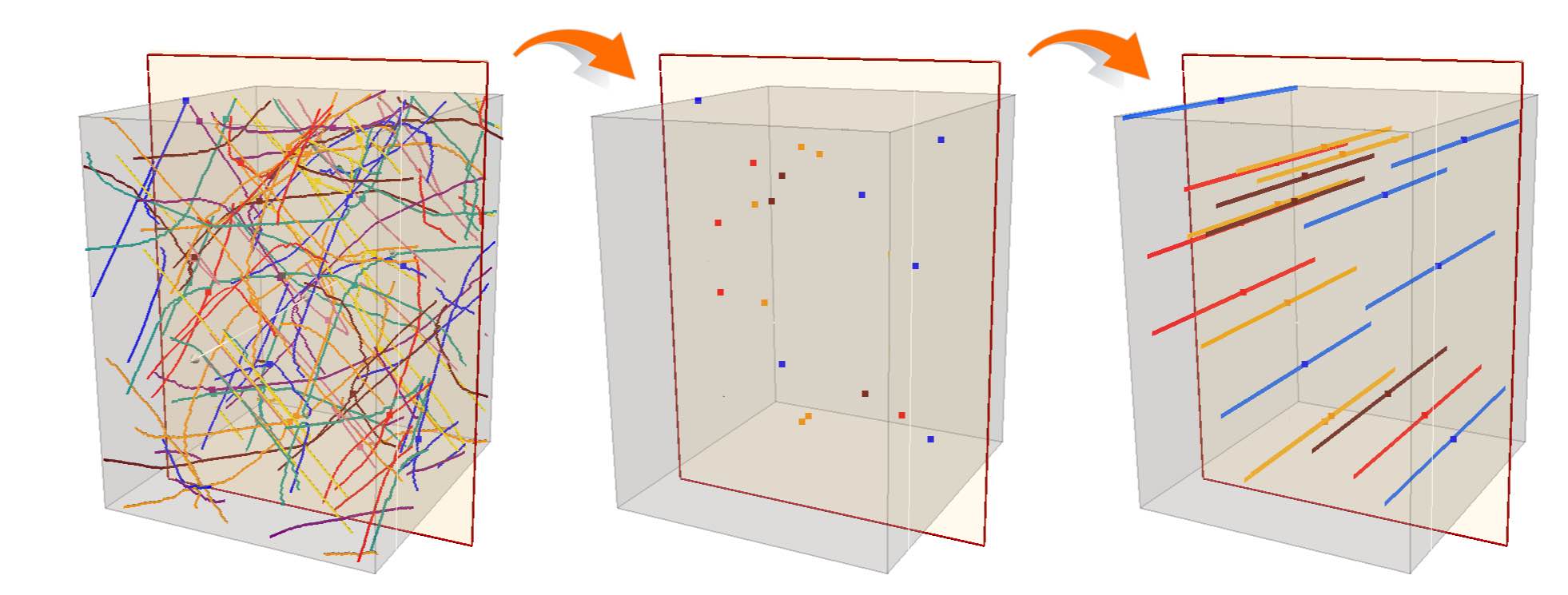
Fig. 2: From 3D to 2.5D dislocation dynamics simulations. In a 3D volume dislocations appear as curved dislocation lines moving in their respective glide planes. If we focus on a 2D reference plane, i.e. a cross section of a 3D volume (red square in the figure), dislocations cross such plane in discrete points. In the 2.5D-DD approach we approximate dislocations in these discrete positions as parallel straight segments and we follow their motion in the 2D reference plane.
Dislocations are then assumed to be perfect straight segments perpendicular to the reference plane and parallel to each other, as shown in Fig. 2. Also, we assumed that all the dislocations are edge in character and their Burgers vector lies in the reference plane. As a consequence the Peach-Kohler force is calculated by adopting such dislocation geometry. Additional local rules are use in the 2.5-D approach in order to mimic realistic 3D mechanisms, as dislocation multiplication, junction formation or emission of dislocation from sources. Even if the dislocation geometry is simplified this method has been demonstrated to be an useful tool to address several plasticity problems as dislocation patterning [4] or, more recently, high temperature creep [5,6]. After setting the initial conditions (dislocation initial configuration, applied load, etc...), the simulations consists mainly in the iteration of the following steps:
- Calculation of the forces acting on each dislocation;
- Calculation of the dislocation velocity;
- Time integration and update of dislocation position;
- Calculation of the plastic strain produced;
- Application of local rules.
The forces acting on the dislocations are calculated by using the Peach-Koehler equation, where the effective stress field σ in Eq. 1 is given by the sum of σapp and σint calculated at the dislocation position. Once the forces are known, the velocities are calculated by using a mobility law which describes the dependence of the dislocation velocity on the effective stress. The latter depends on the physical mechanism controlling the dislocation motion and it may vary with the material and the temperature and pressure conditions. It is indeed of utmost importance to characterize the evolution of the velocity of a single dislocation with stress in order to capture the dynamics of dislocations. Typically a mobility law can be extracted from experiments or from atomistic simulations. Once the expression for the velocity of individual dislocation is provided, dislocations are moved in the forces direction by integrating the velocity over a time step. From the dislocation displacements, the plastic deformation produced during a time step is calculated. Finally, local rules that allow one to reproduce dislocation annihilation, multiplication and junction formation are applied (see Refs. [2, 3] for more details).
In the classical formulation of the DD method, aimed at describing plasticity at low/moderate temperatures, dislocation motion is restricted inside the dislocation glide planes. In this case the effective stress acting on dislocations is the shear stress resolved in the glide plane. Within the 2.5-D approach, restricting the motion of edge dislocations inside the glide planes results in moving dislocations along their Burgers vector direction.
At high temperature, diffusion processes become important. Thus, climb, i.e. the motion of dislocation outside the glide plane, which is promoted by the absorption or emission of point defects at the dislocation position, plays a key role in high temperature plasticity. Still, for a vast class of materials, the glide dislocation motion is faster than climb even at high temperature. Under this assumption, the competition between these two mechanisms during creep tests can be addresses in DD simulations by adopting the following procedure, which allows one to resolve both glide–related and climb-related events (see Refs. [4, 5] for more details):
- The creep stress is applied and dislocations are moved by glide following the procedure described above and adopting a small time step Δtg;
- When dislocations reach a a quasi-equilibrium configuration, i.e. the dislocations are “jammed” and the plastic strain rate drastically decreases, dislocations are moved by climb, during a time step Δtc>>Δtg;
- When a climb displacement of one Burgers vector is achieved by at least one dislocation, the time step is switched back to Δtg and dislocations are moved again by glide only till a new “jammed” configuration is reached.
In these conditions the plastic deformation is mainly produced by glide dislocation motion and climb is the controlling mechanism that allows dislocations to bypass obstacles during the deformation process. We say that plastic deformation is controlled by climb-assisted dislocation motion. This kind of behaviour has been recently modelled in Al [4] and olivine [5].
Creep of Olivine: an application of the 2.5-Dimensional Dislocation Dynamics method
In the following we illustrate the contribution of the climb mechanism to high temperature plasticity in olivine. These results have been recently published in Ref. [5].
In Fig. 3 we show the results of a 2.5-D DD simulation, where a constant applied stress of 40 MPa, in uniaxial tensile deformation conditions have been applied. In particular, we compare the results obtained by activating glide and climb simultaneously with the results obtained by allowing dislocations to move by glide only. When climb is active a steady state regime is found and the plastic strain increases linearly with time. On the contrary when only glide is considered after an initial transient the plastic strain produced saturates. The effect of climb is to release dislocations from a “jammed” configuration, i.e. when dislocations are trapped in a quasi-equilibrium configuration, continuously providing mobile dislocations that can further move by glide and produce plastic strain.
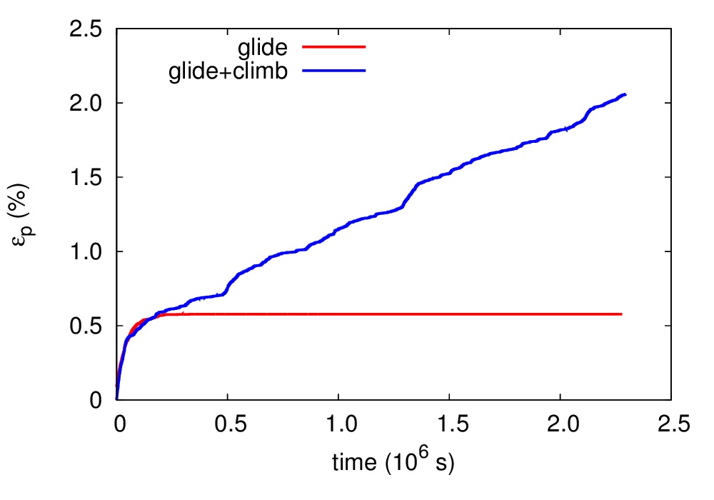
Fig. 3: (a) Strain vs. time curve obtained by including the climb mechanism (blue curve) and by activating the glide mechanism only (red curve).
A sketch of the simulation box and of the loading condition is shown if Fig. 4(a). The tensile loading axis is inclined by 60° with respect to the glide displacement direction, which in our case coincide with the Burgers vector direction. In Fig. 4(b) the initial dislocation microstructure is superimposed to the σyy component of the stress field. The initial dislocation density is 1.4´1012 m-2 and the box size is 8.3 μm. Dislocations with positive (negative) Burgers vector are represented by plus (cross) symbols. Fig. 4(c) and 4(d) show the final microstructure, superimposed to the σyy component of the stress field, obtained when only glide is considered (c) and when both glide and climb are included in the simulation (d). In both cases we can identify dislocation walls perpendicular to the glide direction, as dislocations with the same sign tend to self-organize along this direction. Moreover, we can observe the formation of many dipoles, dislocation couples characterized by the same Burgers vector but with opposite sign. At a given time most of the dislocations are immobile and stored in a dislocation microstructure. Climb allows dislocations involved into dipoles to move outside the glide plane to annihilate or to by-pass repulsive dislocations.
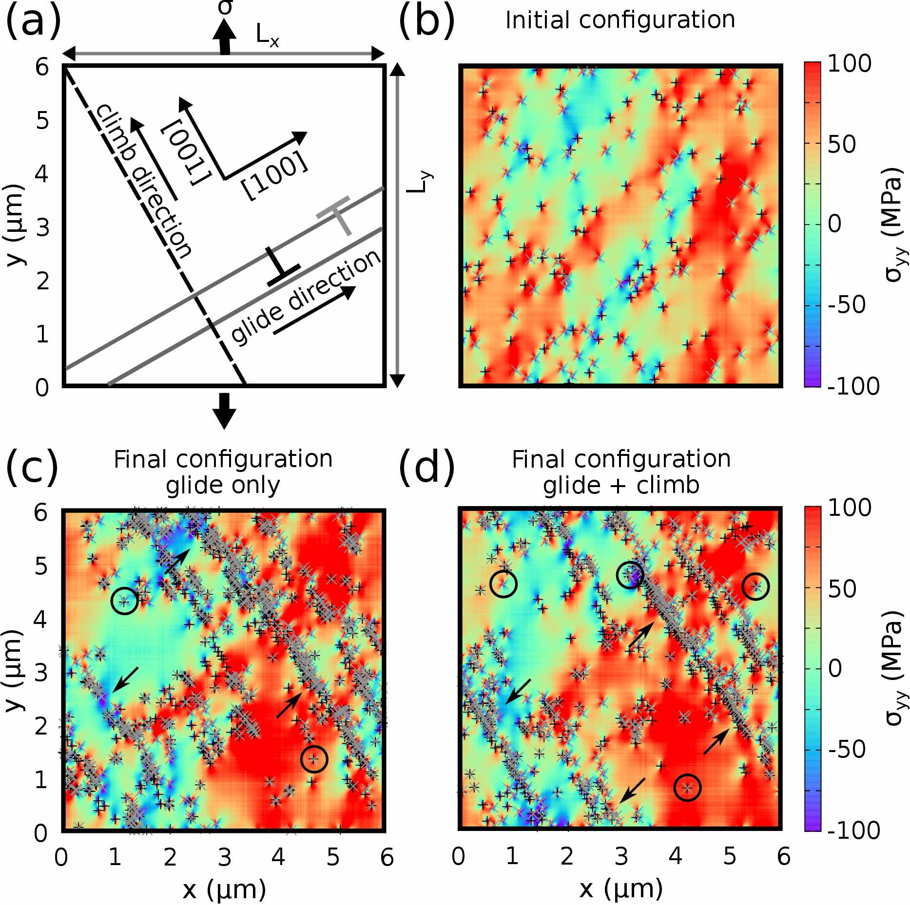
Fig. 4: (a) Sketch of the 2D simulation box. (b-d)Dislocations characterized by positive or negative Burgers vector are indicated with plus or cross symbols. The color background represents the component σyy of the stress field induced by the dislocation microstructure plus the applied external load. (b) Initial dislocation configuration. (c, d) Final dislocation microstructure in a model with glide only (c) and in which glide is coupled with climb (d). Arrows indicate sub-grain boundaries formed by arrays of dislocations and in the circles we can see example of dislocation dipoles.
[1] B. Devincre, R. Madec, S. Queyreau, R. Gatti and L. Kubin, in Mechanics of nano-objects, Paris, Presse de l'Ecole des Mines de Paris, 2011, p. 85.
[2] D. Gomez-Garcia, B. Devincre and L. Kubin, Physical Review Letters, vol. 96, p. 125503, 2006.
[3] A. A. Benzerga, Y. Brechet, A. Needlemann and E. Van der Giessen, Modelling and Simulation in Materials Science and Engineering, vol. 12, no. 1, p. 159, 2004.
[4] S. M. Keralavarma, T. Cagin, A. Arsenlis and A. Benzerga, Physical Review Letters, vol. 109, p. 265504, 2012.
[5] F. Boioli, Ph. Carrez, P. Cordier, B. Devincre & M. Marquille, Modeling the creep properties of olivine by 2.5-D dislocation dynamics simulations. Physical Review B, 92(1) 014115, 2015, doi: 10.1103/PhysRevB.92.014115. Open access