
Electron tomography of dislocations
To model plastic deformation by dislocation dynamics, it is necessary to know the geometry of slip, i.e. the glide, climb and cross-slip planes, amongst others. A good knowledge of the geometry of dislocations interactions is also required.
Electron tomography can be applied to dislocations and gives access to the real 3D structure of a dislocation microstructure.
In most cases, dislocation analyses by transmission electron microscopy (TEM) are limited to Burgers vector identifications, less often to actual characterizations. Full slip systems characterizations are scarce because they are difficult and time-consuming. Actually, the stereographic projection method gives the possibility to find the dislocation glide planes but for one dislocation after the other and with a low accuracy. Dislocation electron tomography allows to get directly the dislocation 3D microstructure and to completely characterize slip systems. Contrary to the stereographic projection technique, the dislocation electron tomography method is accurate and enables fast access to glide planes.
1) Transmitted electron microscope tomography
It is possible to reconstruct a small size objet (from several mm to several nm) in 3D using TEM. TEM gives projected images for different projected angles. These series of images are called « tilted series » (figure 1).
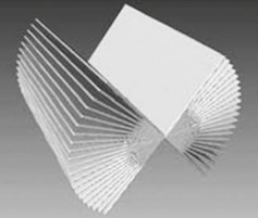
Figure 1: Tilted series.
For usual sample-holders and usual TEM polar pieces gaps, the tilt angle range is lower than +/- 40°. This angular range could reach +/- 60° for high gaps TEM polar pieces and +/- 80° for sample-holders dedicated to tomography. The more the angular range increases, the more the omitted volume (missing wedge) decreases, and the more the reconstruction volume quality rises. Several reconstruction algorithms exist. They are able to transform a tilted series to a stack. Figure 2 describes the weighted back projection (WBP) technique.
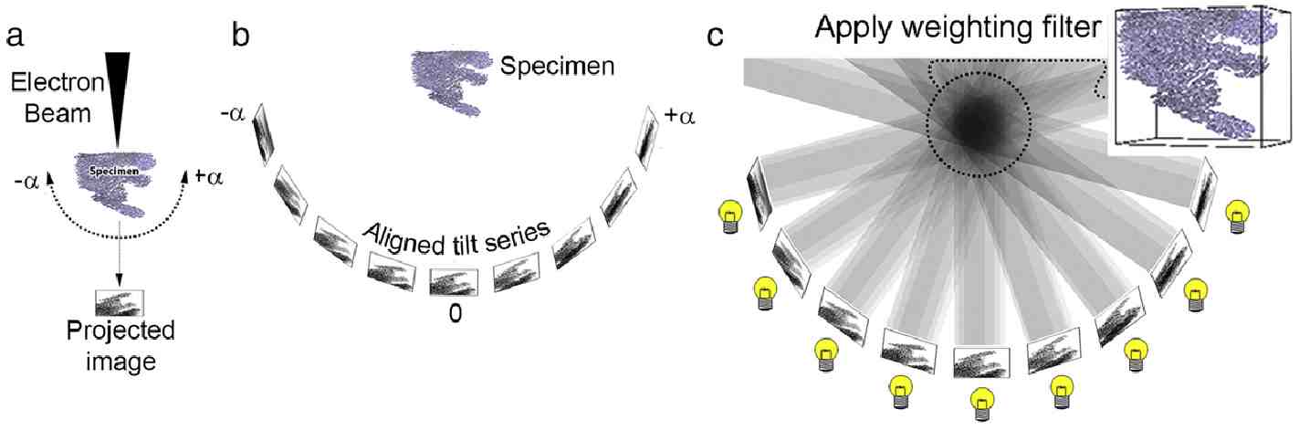
Figure 2 from Liu et al. (Mater. Charact., 2014) : Weighted back projection electron tomography technique.
There are also iterative algorithms as the simultaneous iterative reconstruction technique (SIRT). Figure 3 shows a 3D reconstruction example of a macro-porous zeolite obtained using TEM (Ersen et al. 2007); and figure 4 gives a 3D reconstruction example, from Buseck et al. (2001), of a magnetite nanocrystals obtained using Scanning TEM (STEM).
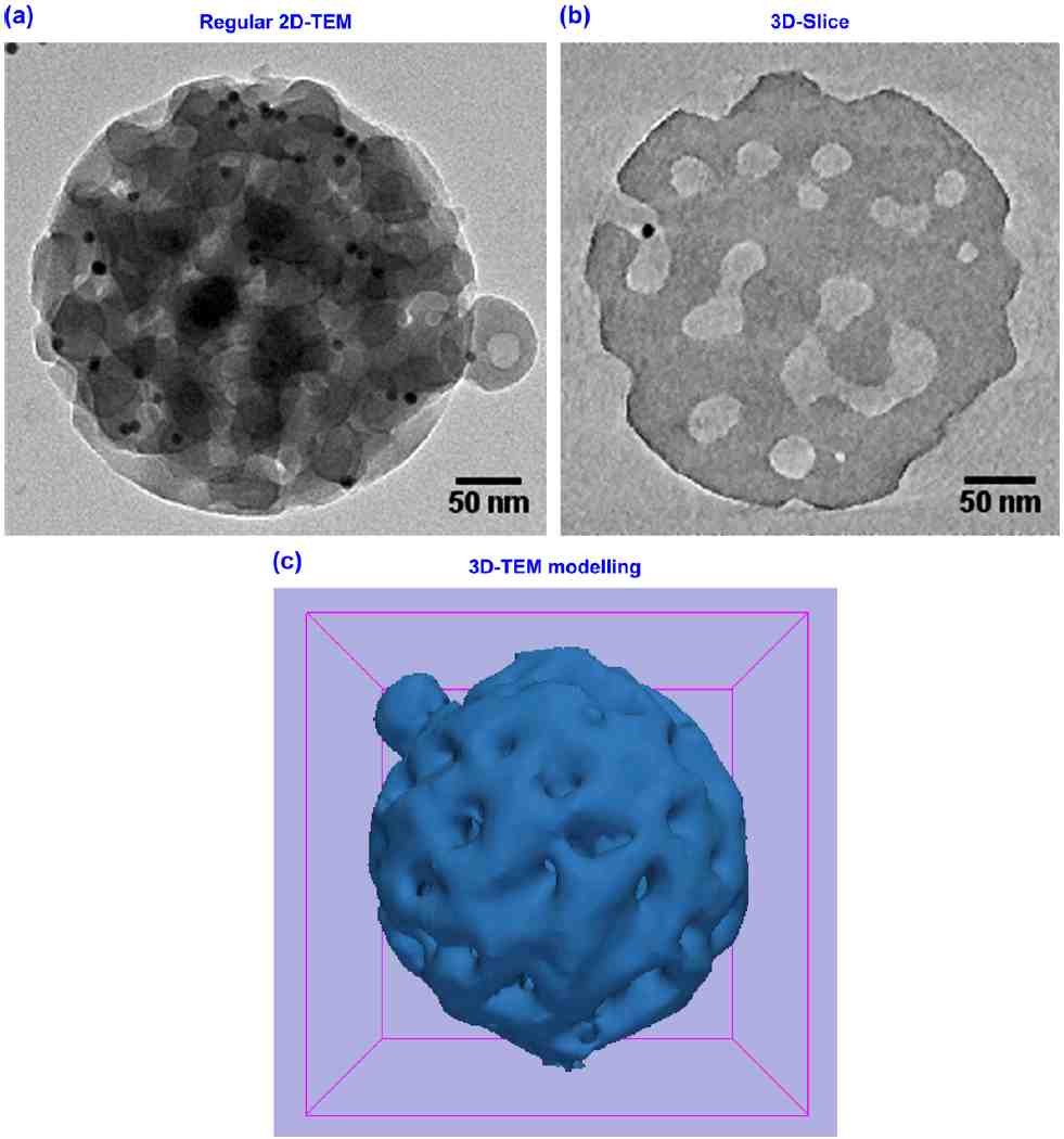
Figure 3 from Ersen et al. (Solid State Sci., 2007): Macroporous zeolite obtained by TEM tomography.
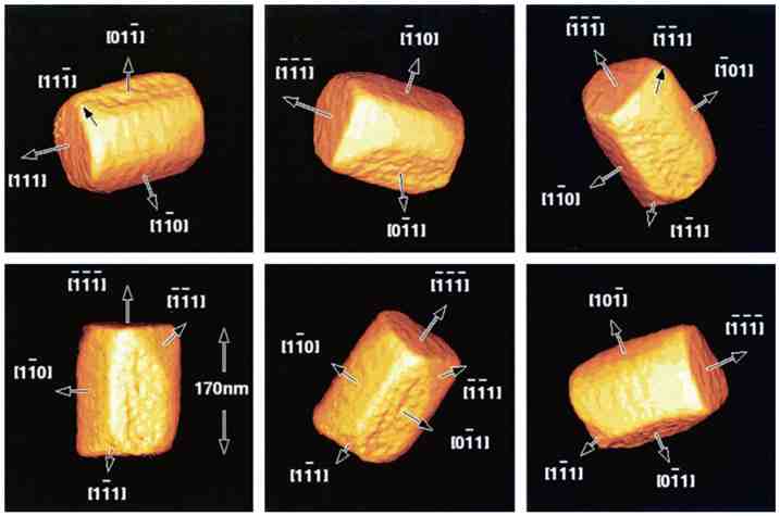
Figure 4 from Buseck et al. (PNAS, 2001): Magnetite nanocrystal obtained by STEM tomography.
2) Transmitted electron microscope tomography of dislocations
The crystallographic plane distortions due to dislocations are the source of dislocation contrasts observed on TEM micrographs. Figure 5 shows the example of an edge dislocation observed with the Bragg angle θB. A small angle deviation (Δθ) gives the possibility to get a high-resolution dislocation image, close to the dislocation core (the resulting image is called a weak beam micrograph).
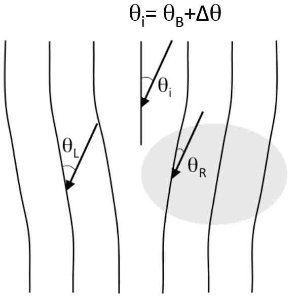
Figure 5: The image is formed by illuminating the sample slightly away from perfect Bragg conditions θi =θB + Δθ; On the right hand side of the dislocation, some distorted planes are oriented in Bragg condition and give rise to a localized diffraction.
Dislocation contrasts are highly linked to the crystal orientation (figure 6).
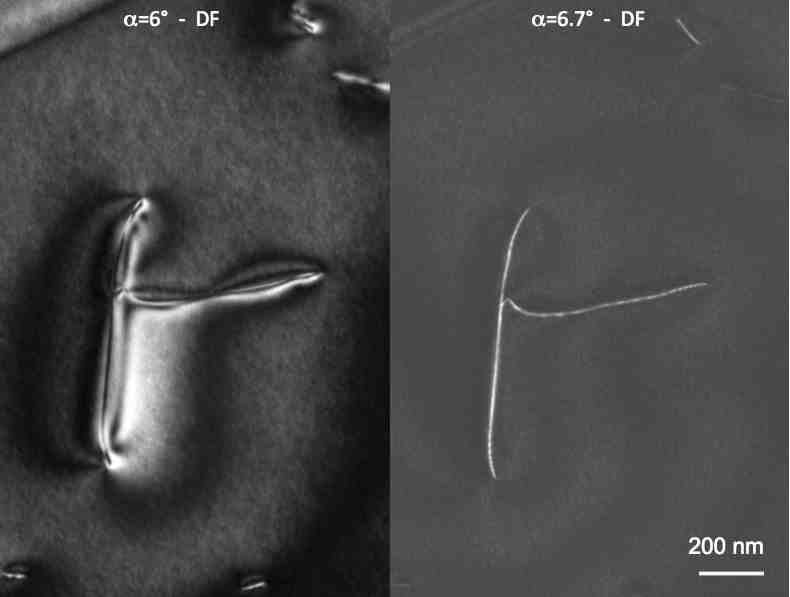
Figure 6: A small angular deviation changes drastically the dislocation contrast and resolution.
Consequently, the specimen needs to be perfectly oriented with the diffraction vector aligned along the tilt axis in order to avoid all Bragg angle variations during the tilted series acquisition (a precision of the order of a tenth of a degree is necessary). Furthermore, the micrographs have to be homogeneous in contrast to get the best 3D reconstruction quality. Two options could be employed:
- the use of a TEM with a field emission gun (FEG);
- the use of a TEM with a LaB6 filament associated with precession (Mussi et al., 2014).
With the first option, the STEM technique allows to obtain a homogeneous contrast (Philips et al., 2011) keeping a high signal over noise ratio. With the second option, acquisitions performed with the TEM weak beam technique gives a high signal over noise ratio. The association of a slight electron beam precession (Vincent & Midgley, 1994) ensures to get homogeneous contrast (figure 7).
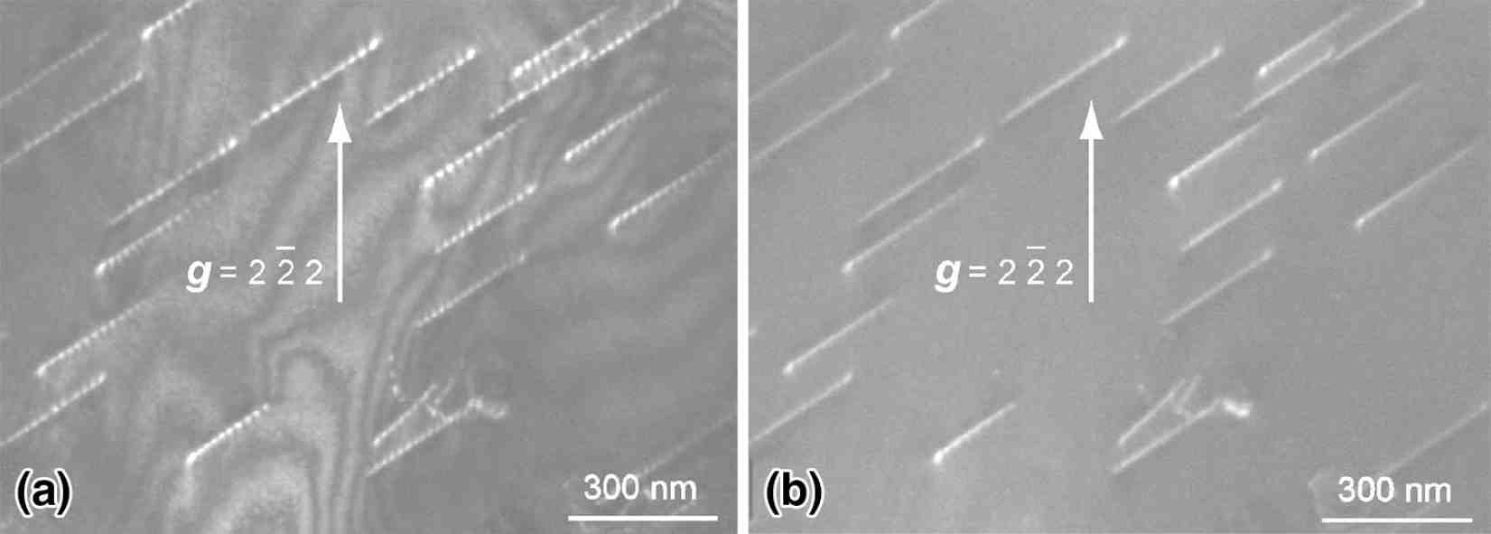
Figure 7 from Mussi et al. (Phys. Chem. Miner., 2014): Contrast homogenization due to an electron beam precession (Rebled et al., 2011).
To increase the dislocation contrast, it is better to filter the tilted series images using for example Kernel filtering and polynomial fit (see figure 8).
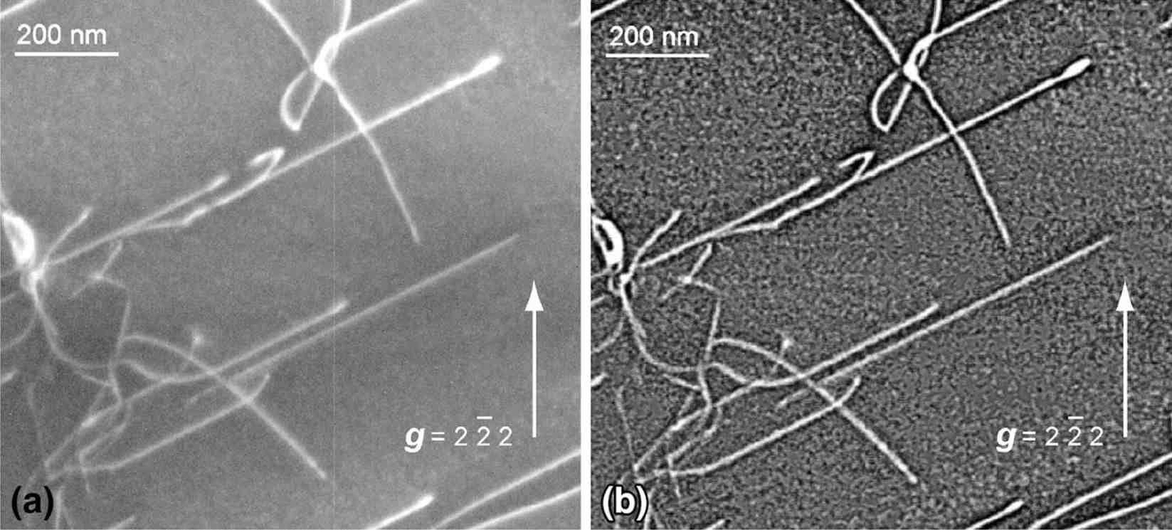
Figure 8 from Mussi et al. (Phys. Chem. Miner., 2014): Dislocation contrast increase due to Kernel filtering and polynomial fit.
We can verify the filtering efficiently on the 3D reconstruction quality on figures 9 and 10.
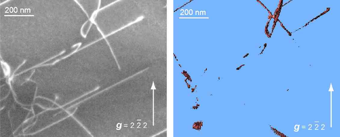
Figure 9 from Mussi et al. (Phys. Chem. Miner., 2014): Unfiltered tilted series and corresponding reconstructed volume.
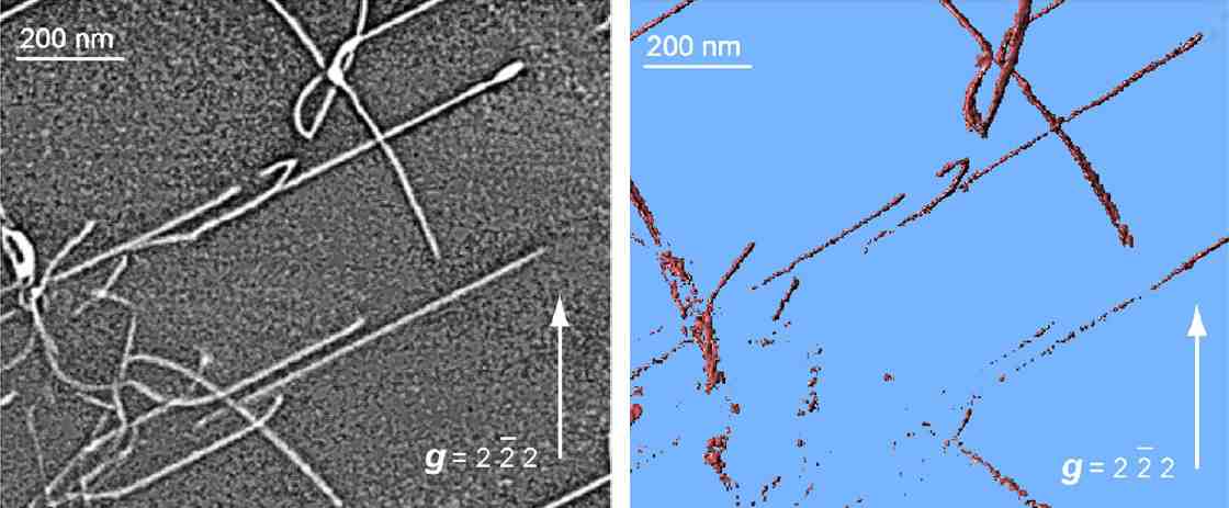
Figure 10 from Mussi et al. (Phys. Chem. Miner., 2014): Filtered tilted series and corresponding reconstructed volume.
All the methodology is described with small movies below (figures 11-15).
Figure 11: Raw tilted series (width: 4 µm)
Figure 12: Tilted series aligned to pixel precision (width: 4 µm)
Figure 13: Filtered tilted series (width: 4 µm)
Figure 14: Corresponding 3D reconstruction (width: 4 µm)
Figure 15: 3D reconstruction with the Chimera visualization software, [100] and [001] dislocations are colored in blue and orange respectively (width: 4 µm)
3) Use of electron tomography of dislocation to characterize the olivine dislocation microstructure at low temperature
At low temperature olivine is plastically deformed by the [001] dislocations glide. A strong lattice friction on screw [001] dislocations is noted in these temperature conditions. Thus, few non-screw dislocation segments are observed on thin foils (see figure 7). Electron tomography is a perfect technique to analyze such a dislocation microstructure.
Examples of glide plane characterization (simple and multiple) and climb plane characterization are described with small movies below (figures 16-18).
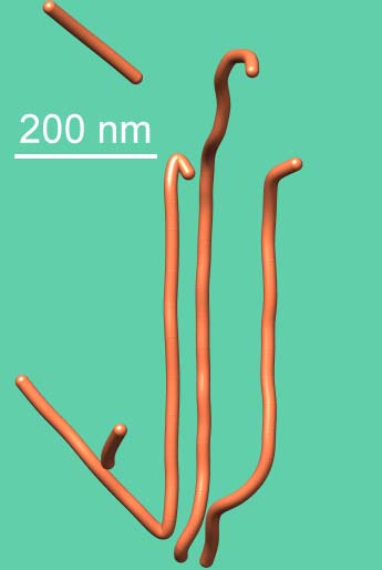
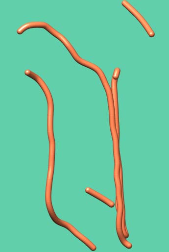
Figure 16: Electron tomographic reconstruction volume showing a (130) glide plane (on the left, the (130) glide plane lies in the projection plane; on the right the (130) glide plane is edge-on)
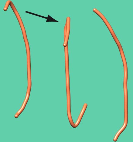
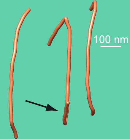
Figure 17: Electron tomographic reconstruction volume showing different glide planes for a single dislocation (on the left, the (010) glide plane of the dislocation segment situated on the top of the volume (see black arrow) is edge-on; on the right, the (140) glide plane of the dislocation segment situated on the bottom part of the volume (see black arrow) is edge-on)
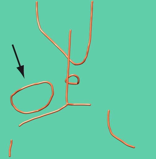
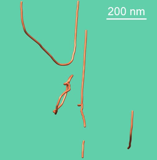
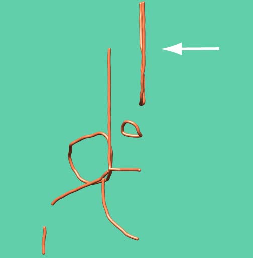
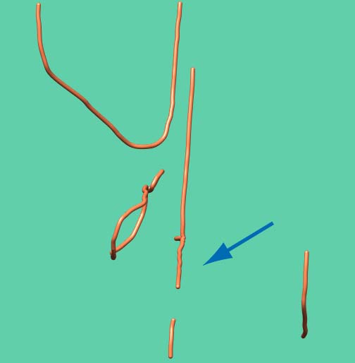
Figure 18: Electron tomographic reconstruction volume showing glide planes and a sessile loop lying on a climb plane (on the extreme left, the lying plane of the dislocation loop lies in the projection plane (black arrow); on the left, the lying plane of the dislocation loop is edge-on; on the right, the (110) glide plane is edge-on (white arrow); on the extreme right, the (1-10) glide plane is edge-on (blue arrow))
References:
P.R. Buseck, R.E. Dunin-Borkowski, B. Devouard, R.B. Frankel, M.R. McCartney, P.A. Midgley, M. Pósfai, M. Weyland (2001) Magnetite morphology and life on Mars. Proc Natl Acad Sci USA 98:13490–13495.
O. Ersen, C. Hirlimann, M. Drillon, J. Werckmann, F. Tihay, C. Pham-Huu, C. Crucifix, P. Schultz (2007) 3D-TEM characterization of nanometric objects. Solid State Sciences 9:1088-1098.
G.S. Liu, S.D. House, J. Kacher, M. Tanaka, K. Higashida and I.M. Robertson (2014) Electron tomography of dislocation structures. Mater. Charact. 87 :1-11.
A. Mussi, P. Cordier, S. Demouchy, C. Vanmansart (2014) Characterization of the glide planes of the [001] screw dislocations in olivine using electron tomography Phys. Chem. Miner. 41:537-545.
P.J. Phillips, M.C. Brandes, M.J. Mills, M. De Graef (2011) Diffraction contrast STEM of dislocations: imaging and simulations. Ultramicroscopy 111:1483–1487.
J.M. Rebled, L. Yedra, S. Estrade, J. Portillo, F. Peiro (2011) A new approach for 3D reconstruction from bright field TEM imaging: beam precession assisted electron tomography. Ultramicroscopy 111:1504–1511.
R. Vincent & P.A. Midgley (1994) Double conical beam-rocking system for measurement of integrated electron diffraction intensities. Ultramicroscopy, 53, 271–282.
M. Weyland, P.A. Midgley, R. Brydson, A.R. Lupini, S.N. Rashkeev, M. Varela, A.Y. Borisevich, M.P. Oxley, K.V. Benthem, Y. Peng, N.d. Jonge, G.M. Veith, S.T. Pantelides, M.F. Chisholm, S.J. Pennycook, R.E. Dunin-Borkowski, T. Kasama, R.J. Harrison, D.J. Smith, P.L. Gai, M.R. Castell (2007), Nanocharacterization, RSC Publishing.
D.B. Williams & C.B. Carter, in Transmission Electron Microscopy: A textbook for materials science (Plenum Press, 2nd edition, 2009).
Movies: